Building the Foundation for Unit Economics at an AI Infrastructure Company
This post covers building COGS infrastructure for AssemblyAI, a leading global Voice AI company.

Thesis: For AI infrastructure providers, relying on the monthly invoices provided by cloud providers is structurally insufficient to support the decisions Engineering, Sales, and Finance need to make. Accurate cost-of-goods-sold (COGS) and unit economics for an AI infrastructure company requires a methodology that joins multiple incomplete billing data sources to fill in crucial gaps in reporting, allocates compute cost via cascading layers, and buckets costs into capacity classes highlighting areas of opportunities for cost efficiencies. This process involved incorporating documented methodology from credible sources - such as AWS - in addition to creating proprietary methodology designed for AssemblyAI. The purpose of this post is to share how we went about this as part of an effort to help shape how the AI industry defines unit economics.
It’s the year 2026 and there is no shortage of content about managing your AI spend. FinOps practitioners, cloud vendors, and tooling companies have produced a steady stream of guides on how to allocate ChatGPT token costs to business functions, how to right-size GPU clusters, how to set budget alerts before a runaway agent empties your credit card, and so on. This isn’t just anecdotal chatter anymore either; it’s a clear signal of a significant structural shift in the industry. For instance, at the upcoming FinOps X conference in June 2026, nearly a third of the agenda is now dedicated exclusively to AI - transforming the conversation into a formalized discipline of AI cost transparency and value management.
Yet, for all this momentum in better understanding how to allocate AI spend, this post is about the other side of that equation - a perspective that’s almost entirely absent from public-facing literature within the intersection of FinOps and AI at the time of writing this.
AssemblyAI is, at its core, an AI infrastructure company. We build and train our own models and provide them - alongside a wide variety of third-party large language models - to developers and companies all over the world who are building applications on top of our state-of-the-art Voice AI products. A common scenario is as such: a customer makes an API call, the call runs on our infrastructure and gets transcribed by one of our models, and then at the end of the month we get charged by AWS. Within the AI infrastructure industry, the problems are more nuanced than just “how much are we spending?” - which companies can deduce from their monthly invoices - but they also include challenges such as “how can we allocate costs on a shared production infrastructure?”, “how is that cost trending as our infrastructure evolves?”, and “where are the highest-leverage optimization opportunities in our infrastructure footprint?” Building the data infrastructure to answer questions like these - confidently, repeatably, and at the granularity decisions actually require - goes beyond the scope of what a monthly AWS invoice can do.
To answer these questions and then some, one must understand how to best define what unit economic metrics are most valuable, such as cost per audio hour by speech model, cost per token across LLM-powered features, or cost per request across language combinations. To simply provide a single cost figure as a numerator and a single audio hours figure as a denominator has the potential to obscure inefficiencies unknowingly inflating the bottom line. The compute cost an ECS task consumes while running, the cost of the unused capacity reserved alongside it inside the same instance, and the cost of taskless instances kept warm for capacity planning are causally distinct kinds of cost invisible within the raw unit economic numbers. To avoid this, we built a methodology that decomposes our unit economics into three distinct classes - in-use, idle reserved, and dark reserved - each defensible as a separate number. The decomposition itself isn’t well-documented in public literature as far as we’ve been able to find, but recent production behaviors have aligned closely with what the methodology predicted - which gave us confidence the three-class framing reflects real operational reality rather than just an accounting convenience.
For AssemblyAI in particular, these are increasingly hard questions to answer when your production infrastructure spans multiple production regions, several product lines, and a fleet of compute workers - some serving single or multiple models, languages, and customers simultaneously. And as someone who has spent the better part of the last few years building the data models to answer them, I’ll be first to say: cleaning up the millions of nebulous billings records is the easy part. Defining unit economics and providing COGS figures that stakeholders trust and actually act on is a different kind of problem entirely.
How I Ended Up Here
I inherited this challenge in early 2024, a few months after onboarding at AssemblyAI. What I received from an outside consultant who had previously owned it - with help from Engineering - was a cost model that worked for the scope it was intended to serve: where are our infrastructure costs going at a product level? But it was difficult to read and understand, practically impossible to scale, and built upon AWS’s Cost and Usage Report (CUR) 2.0 in ways that created a hard ceiling on accuracy.¹
The specific problem we needed to solve: accurate amortized costs at the resource level. AssemblyAI partners with AWS on long-term capacity commitments via Savings Plans (SP) that reduce our effective compute rates. CUR 2.0 handles SP discounts as a separate line item adjustment rather than attributing the discount at the point of resource usage, which meant the pipeline had to derive amortized costs through a chain of scaling calculations - over five CTEs worth of SP math that produced workable totals but couldn’t produce the per-resource effective cost we wanted at the granularity our analysis required.
In late 2025 I came across the FinOps Foundation - a year later than I’d like to have done so - and their FOCUS 1.2 specification.² FOCUS introduced the concept of EffectiveCost: true per-resource amortized cost, calculated at the point of attribution rather than as an after-the-fact adjustment. Shortly thereafter, when AWS released native FOCUS 1.2 data exports, the aforementioned ceiling we had been pushing against was finally gone.³ Or so we thought.
Contrary to the typical shift-and-lift migration that some FinOps Practitioners recommend, we came to realize that the new FOCUS dataset couldn’t truly replace CUR within our data models, and that’s a distinction worth calling out. While FOCUS 1.2 contains 61 standard FOCUS columns plus three AWS extensions, the split_line_item_* columns - truly integral data components for AssemblyAI due to our production infrastructure - that CUR uses for per-task ECS cost attribution didn’t exist in FOCUS. Given that FOCUS is meant to be a cross-cloud standard, this was by design and it’s understandable that provider-specific extensions like Split Cost Allocation Data (SCAD) live outside it, which means that SCAD as of today is strictly a CUR-specific feature.⁴
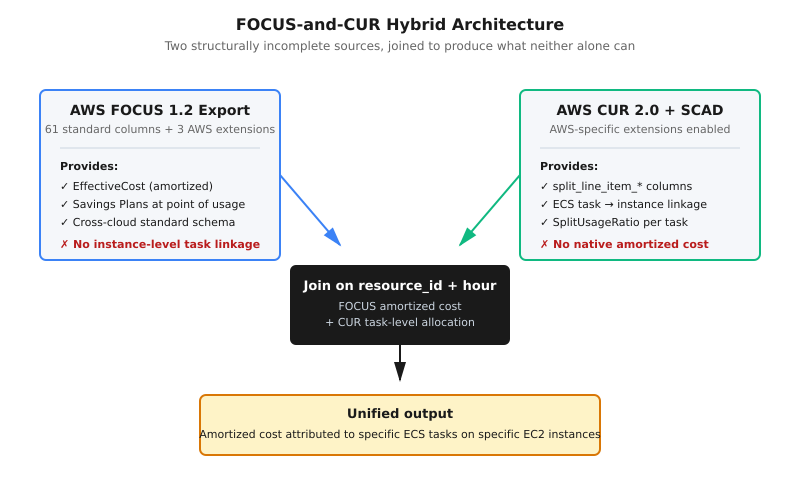
The end result: the pipeline we eventually graduated to reads from both sources and joins them: FOCUS for the amortized EffectiveCost and CUR for the SCAD instance-level task linkage. Each source is structurally incomplete on its own for what we need. However, together they give us what neither alone can: amortized cost attributed to specific ECS tasks running on specific EC2 instances, including the instances that serve our speech models.
Why Does This Even Matter?
Pricing decisions in AI infrastructure get made on a faster timeline than cost attribution can keep up with. New model launches, capacity reallocations, and shifts in customer mix all change the underlying cost structure in ways that the billing data takes weeks to fully reflect. During those windows, pricing teams are implicitly asking questions the cost data can’t yet answer: are pricing assumptions holding up against actual cost behavior? Are there optimization opportunities the team hasn’t caught yet? How quickly can the cost infrastructure catch up when the product moves faster than the data does?
These aren’t hypothetical concerns. They’re the daily operational reality of running an AI infrastructure business at scale - and they’re a meaningful piece of why the data infrastructure has to be built before the product needs it, not after.
Voice AI is a competitive market, and unit economics aren’t just internal reporting metrics. They’re the foundation of every pricing conversation, every decision about which models to prioritize for optimization efforts, every judgment call about whether expanding into a new region makes financial sense. Fine-tuning our unit economics isn’t a one-time exercise. It’s an increasingly strategic one, and it’s an ongoing one - the methodology continues to get refined as the business evolves.
Defining Unit Economics for a Voice AI Company
Before you can build the infrastructure to calculate COGS, you have to agree on what you’re actually trying to measure. Several questions need explicit answers:
What is the unit - and which unit? For our core speech-to-text products, the natural unit is an audio hour - not compute time consumed. This is the core metric that makes cost per unit interpretable across model versions: if a new model processes audio faster but the same number of hours flows through the pipeline, cost-per-unit movements reflect real cost efficiency changes rather than throughput noise.
For our LLM-powered products, the unit is tokens, which posed a challenge given that cost per audio hour and cost per token aren’t easily reduced to a common unit. When a customer uses a product that chains speech recognition with an LLM, you have two cost denominators that don’t share commonalities. We track them separately, which means unit economics for hybrid products requires special handling unique to the combination involved.
What costs belong in COGS? Accurate COGS also requires organizational visibility that pure data work can’t provide on its own. Knowing whether a model’s costs should be classified as production or pre-launch requires knowing when a product actually went GA - which means that we need to track product launch calendars, not just billing data. Finance, Analytics, and Engineering have to be talking to ensure we’re correctly tagging which costs should be pulled into COGS and which should be allocated to R&D.
How do you handle the anomaly problem? Accurate numbers can still raise questions when context isn’t visible alongside them. A service line migrating infrastructure mid-quarter shows inflated costs for that period. A new model with low initial traffic has disproportionately high per-unit costs because fixed compute is spread over fewer hours. If you can’t tell that story - here’s the worker, here’s the transition timeline, here’s why this cost spike is temporary - you lose stakeholder trust quickly. When we deployed the most recent version of our calculations, we maintained confidence by running two parallel conversations: explaining anomaly stories using Looker dashboards that show worker-level cost trajectories alongside traffic patterns, and demonstrating that total cost figures reconcile exactly against what teams could see in AWS Cost Explorer. Both were necessary. Neither was sufficient alone.
Triple-Layer Allocation
Even with the FOCUS-and-CUR pipeline producing clean amortized costs at the resource level, the harder problem remained: distributing that cost across the products, models, and languages that share the same infrastructure.
For a Voice AI company, the infrastructure is fundamentally shared and multi-tenant at every layer. When a customer submits an audio file or starts a streaming session with AssemblyAI, that request moves through a sequence of workers performing speech model inference and sometimes additional features such formatting and speaker diarization, which are all running in shared ECS clusters simultaneously serving requests from thousands of other customers, across multiple language models, feature combinations, and AWS regions. The bill reflects none of that. It simply states “Amazon EC2 — Compute Optimized, us-west-2.” There’s not much we can do with that.
This led to the creation of our triple-layer allocation method, with each layer building upon the previous one:
Layer 1: Attributing compute costs to workers. Some instances run multiple models. Some support multiple languages. Some only support one of each. And that doesn’t cover all of the combinations available. The billing data knows about the instances; however, it doesn’t know which ECS service ran on it, in what proportion, for how long, and so on.
Therefore, we have to incorporate attribution logic which breaks into two cases depending on instance type.
For non-GPU instances, CUR’s SCAD feature handles this directly via a documented 9:1 CPU-and-memory ratio derived from AWS Fargate pricing.⁵ This is the well-supported path - apply SCAD, get task-level attribution, move on.
For GPU instances, SCAD’s accelerated-instance allocation is currently focused on EKS, and we run on ECS. To extend the SCAD pattern to our environment, we derive empirical GPU rates from comparable on-demand pricing and apply dimensional allocation across (GPU, vCPU, memory). We’re working in tandem with AWS on ECS GPU cost attribution as a feature area they’re actively developing, which will help us continue to refine our current methodology even further.
Once costs land at the ECS service level, a final allocation step remains: the cost for a single worker must be further split between models, languages, etc., proportional to actual hourly usage, with a cold-start fallback for new configurations that don’t yet have usage history. Again, this is to ensure that no costs get silently dropped.
Layer 2: Distributing shared services across product lines. Beyond compute, there are dozens of AWS services that support the entire platform without mapping cleanly to any individual product, representing a meaningful portion of total infrastructure spend. Each gets determined by what causal signal is available for a given service:
Services with AWS tag coverage get distributed directly to the product line identified by the tag.
Services that scale with API request volume are distributed by request count, with infrastructure-intensity weights that account for the fact that some product lines generate more infrastructure load per request than others.
Services that scale with container presence use container-count proportional distribution.
Fixed-cost services with no causal usage metric are distributed by even split across product lines.
Everything else falls through to audio-hour proportional distribution as the general fallback.
The distribution cascade has an explicit zero-weight guard at every tier to prevent fall-through: a service row that matches a tier’s condition but has zero usage metric receives weight zero rather than leaking into lower tiers. This ensures the total distributed cost equals the input cost by mathematical construction - not as an approximation, but as a guarantee to ensure no costs get dropped.
Layer 3: Allocating costs to languages. Within a given product and model, costs need to be attributed to the languages being processed. Language mix varies by region, shifts as new languages launch, and affects the cost structure of some models more than others. We handle this using an internally-defined time-bound rolling window of actual audio hours by language, region, and speech model - long enough to smooth day-of-week and holiday variances, short enough to reflect real traffic shifts when a new language launches. Every allocation path is designed to degrade gracefully when data doesn’t exist yet: if no usage history is available for a new model or language, the pipeline falls back to an even split rather than misallocating costs.
One of the more clarifying moments in building this pipeline came when an engineering lead pointed out, mid-conversation about our allocation approach for a newly-released model, that one particular service was consuming a specific AWS product at a completely different rate than the others, which wasn’t being reflected in our calculations. It only became visible when we started looking at tag-level usage data allocated by team. That was a humbling realization which changed the architecture of the shared service distribution layer entirely - and it’s a good example of why this problem requires ongoing transparent collaboration with engineering, not just a one-time data modeling exercise.
The result of all three layers: a pipeline that produces cost data at the grain of (hour × product × speech model × language × AWS region), which serves as the foundation for our unit economics.
Class Capacity Framework
The triple-layer allocation gives us the foundation: cost data at meaningful granularity, attributed to the right consumers. The class capacity framework gives us the diagnostic layer on top of that foundation. Once you have unit economics at the right grain, the next question is invariably 'why did that number move?' - and answering it requires decomposing the underlying compute cost into the operational levers that actually drive change.
The pipeline now decomposes compute cost into three causally distinct capacity classes:
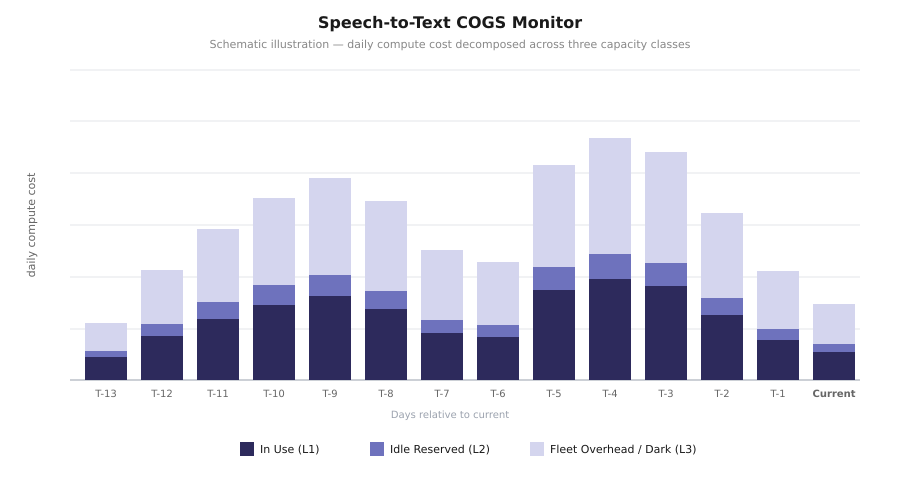
In-use: what an ECS task actually consumed while running.
Idle reserved: unused capacity within an instance that has tasks running on it.
Dark reserved: taskless instances kept warm for capacity planning.
These three classes are causally distinct, not just accounting conveniences. They represent fundamentally different optimization levers - in-use cost is sensitive to workload efficiency, idle reserved is sensitive to per-instance utilization, and dark reserved is sensitive to fleet provisioning. Rolling them into a single number means you can’t tell whether your unit economics moved because workloads got more efficient, capacity utilization improved, or fleet provisioning changed.
Operationally, this decomposition has been transformational for how we read cost movements. A unit economic change that looks like a single anomalous bar in a Looker dashboard now decomposes into a much more readable story: did the underlying workload get more or less efficient? Did capacity within active instances become better or worse utilized? Did fleet provisioning change at the product level? Each of those questions maps cleanly to one of the three classes, and answering them no longer requires manual investigation into the underlying ECS data. The methodology turns 'what’s this anomaly in the cost data' from a multi-hour investigation into a structured diagnostic process that takes minutes.
The methodology draws on AWS-native patterns where they exist - SCAD’s UnusedCost × SplitUsageRatio approach for idle attribution within instances - and on AssemblyAI-curated methodology where AWS-native patterns don’t yet exist, particularly fleet-based attribution for dark capacity with daemon-task exclusion.
What makes this framework different from typical cost-attribution approaches is that it doesn't just allocate cost - it explains it. The three classes don't change the total compute spend by a single dollar. They change what the spend means. A team looking at a 15% cost increase month-over-month can now see whether that increase came from serving more traffic (in-use cost rising), serving the same traffic less efficiently (idle reserved rising), or provisioning ahead of demand that hasn't materialized yet (dark reserved rising). Each of those scenarios requires a different operational response, and none of them are visible from the aggregate cost number alone.
What This Infrastructure Unlocks
After multiple iterations of our models, each one a meaningful step forward in refining what the methodology could measure - built on top of an illegal amount of coffee and a continuous feedback loop of “is this allocation approach defensible?” - we landed on a methodology that produces unit economics that don’t just represent the current state of our costs, but also help tell the story behind them.
It’s worth being concrete about the output, because it shapes what questions you can and can’t answer. As a result, the pipeline produces a table refreshed on a daily basis at the grain of (hour × product line × speech model × language × AWS region) that allows us to dive into resource consumption behaviors. For a company like AssemblyAI, this produces a granular but queryable dataset that answers questions such as:
What is the cost per audio hour for a specific async transcription model in a specific region over the trailing 30 days, and how has it trended month-over-month?
How does the cost per audio hour for a given model compare between EU and NA regions, and what explains the gap?
Which compute workers account for the largest share of cost in a specific product line, and are any of them growing disproportionately to volume?
When a new model launches, what are its unit economics compared to the model it’s replacing?
The same data feeds three distinct consumers with different needs: Finance is able to reference monthly rollups for COGS reporting and trend analysis. Engineering uses the worker-level detail to own the cost consequences of infrastructure decisions. Customer Success uses the model-and-region-level unit cost rates as a reference point in enterprise pricing conversations.
Getting all three of those stakeholders to trust the same numbers - while using them for different purposes - is, in some ways, the hardest part of the whole project.
There’s also a customer-facing dimension to this work that’s worth naming directly. Accurate unit economics are what make it possible to invest deliberately in the parts of infrastructure that customers actually feel - reliability, latency, the ability to ship state-of-the-art models at production scale. They’re also what let pricing stay predictable and durable. For customers depending on us as a critical infrastructure provider, the value of this work shows up most in what it enables us to do: confidently invest in the model quality and infrastructure reliability that makes us a trusted choice for production AI workloads.
Building the foundation for unit economics doesn’t just produce numbers - it produces metrics that can carry the weight of the decisions made on top of them. For an AI infrastructure company tripling revenue in a year and scaling rapidly, that’s not a back-office convenience. It’s a competitive prerequisite.
Questions, pushback, or your own war stories on this: I’m most reachable on LinkedIn. This is a hard problem with no single right answer, and the most useful thing I’ve built is an opinionated approach - not a universal one.
References
Amazon Web Services. AWS Cost and Usage Reports. AWS Documentation. https://docs.aws.amazon.com/cur/latest/userguide/what-is-cur.html
FinOps Foundation. FOCUS Specification v1.2. Joint Development Foundation Projects, LLC. Ratified May 29, 2025. https://focus.finops.org/focus-specification/v1-2/
Amazon Web Services. Creating data exports for the FOCUS 1.0 dataset. AWS Documentation. https://docs.aws.amazon.com/cur/latest/userguide/dataexports-create-focus.html
Amazon Web Services. Split cost allocation data for AWS billing. AWS Documentation. https://docs.aws.amazon.com/cur/latest/userguide/split-cost-allocation-data.html
Amazon Web Services. Example of split cost allocation data calculations. AWS Documentation. https://docs.aws.amazon.com/cur/latest/userguide/example-split-cost-allocation-data.html